Introduction
In 2022, CAMAG laboratory introduced the concept of complementary developing solvents (CDS) based on the combination of three automated analyses using three developing solvents (DS): one low polarity (LPDS), one medium polarity (MPDS), and one high polarity (HPDS) solvent [1]. With these three DS, any compound is characterized by three RF values instead of one. Introduced into a database, a large dataset can be compiled from these values, which then may be subjected to data mining and machine learning.
In their paper [2], CAMAG researchers describe how the application of a CDS protocol to a large number of highly diverse individual compounds was used in combination with machine learning to predict the RF values of individual substances from molecular properties, and to generate proposals for the identity of a zone. Coupled with machine learning, the CDS concept as a very powerful, general, and medium to high throughput technique for routine analysis and sophisticated research, may become the future of HPTLC. It may help replacing common tasks such as visual evaluation and pattern recognition, as well as subjective pass/fail decisions by automated procedures and numerical values generated by suitable algorithms.
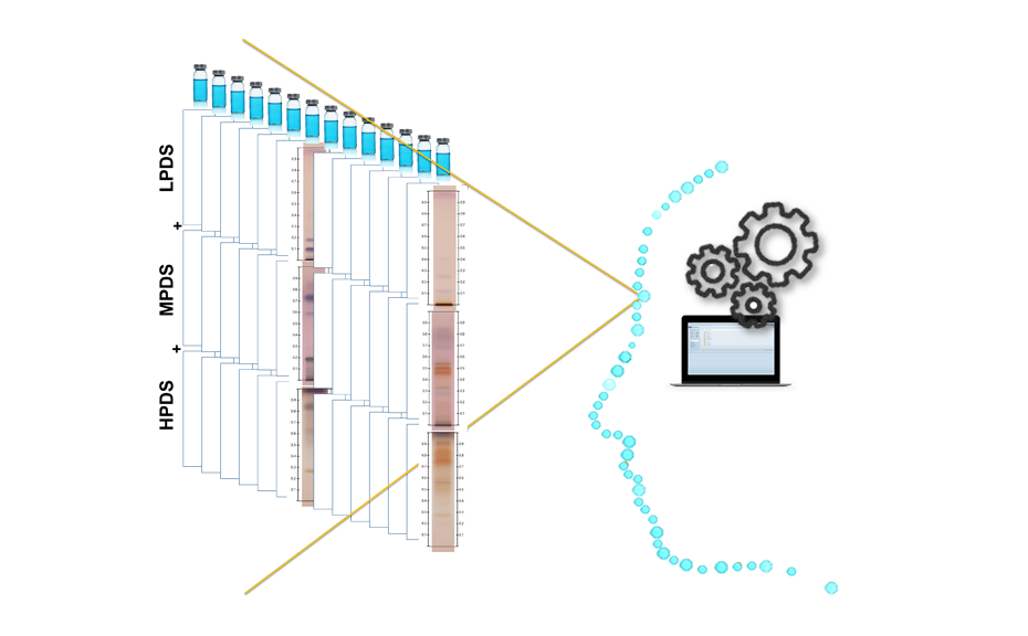
Visualization of the CDS and its composite fingerprint
Standard solutions
Individual standard solutions were prepared at a concentration of 1.0 mg/mL (adjusted when necessary). Methanol was used as solvent for iridoids, coumarins, pharmaceutical drugs, flavonoids, triterpenes, sesquiterpenes, steroids, phospholipids and cannabinoids, 50% aqueous acetonitrile for carbohydrates, 50% aqueous methanol for amino acids, and toluene for monoterpenes. System Suitability Test (SST): the ready to use solution of Universal HPTLC Mix (UHM) was prepared in house according to [3] and applied on each plate.
Chromatogram layer
HPTLC plates silica gel 60 F254 (Supelco/Merck), 20 x 10 cm are used.
Sample application
2.0 μL of sample solutions are applied as bands with the Automatic TLC Sampler (ATS 4), 15 tracks, band length 8.0 mm, distance from left edge 20.0 mm, distance from lower edge 8.0 mm.
Chromatography
Plates were developed with the three developing solvents in the ADC 2 with activation of the plate at 33% relative humidity for 10 min using a saturated solution of magnesium chloride. LPDS (toluene, ethyl acetate 9:1 (V/V)) is used without saturation, whereas MPDS (cyclopentyl methyl ether, tetrahydrofuran, water, formic acid 40:24:1:1 (V/V)) and HPDS (ethanol, dichloromethane, water, formic acid 16:16:4:1 (V/V)) are used with 20 min chamber saturation (with saturation pad). The developing distance for all three methods was 70 mm (from the lower edge). Plates were dried for 5 min.
Post-chromatographic derivatization
Derivatization with anisaldehyde sulfuric acid reagent (10.0 mL of sulfuric acid were carefully added to the ice-cold mixture of 170.0 mL of methanol and 20.0 mL of acetic acid. To this solution, 1.0 mL of anisaldehyde was added) by spraying (Derivatizer, blue nozzle, 3.0 mL, spraying level 3) was followed by 3 min of heating at 100°C. Images of plates derivatized with Fast blue salt B reagent (250.0 mg of Fast blue salt B (o-dianisidine bis(diazotized) zinc double salt) were dissolved in 10.0 mL of water and mixed with 25.0 mL of methanol and 15.0 mL of dichloromethane) were captured within 2 min after spraying (Derivatizer, green nozzle, 3.0 mL, spraying level 5).
For the derivatization with NP reagent (1.0 g of diphenylborinic acid aminoethylester was dissolved in 200 mL of ethyl acetate ) / PEG (10 g of polyethylene glycol 400 (macrogol) were dissolved in 200 mL of dichloromethane), the plates were heated at 100 °C for 3 min, cooled to room temperature, then sprayed with the mixture NP/PEG 1:1 (V/V) (Derivatizer, green nozzle, 3.0 mL, spraying level 3), and dried for 2 min. Derivatization by immersion (Immersion Device, speed 5, time 0) with toluene sulfonic acid reagent (10% of p-toluene sulfonic acid in ethanol) was followed by heating at 150°C for 3 min.
Documentation
TLC Visualizer in UV 254 nm, UV 366 nm, and white light prior to derivatization, and UV 366 nm, and white light after derivatization (as needed).
Densitometry
For the UHM, TLC Scanner 4 and visionCATS, absorbance measurement at 254 nm, slit dimension 5.00 mm x 0.20 mm, scanning speed 50 mm/s, and in fluorescence mode at 366>/400 nm.
Numerical databases preparation and processing
The open-source software KNIME (version 4.6) was used. The “RDKit KNIME Integration” was applied for curation of the databases and conversion of the chemical structures. 178 chemicals of the learning set were then used to benchmark various machine learning models.
Machine learning
RF values obtained from peak profiles from images (PPI) or scanning densitometry (PPSD), were used with the Random Forest regressor algorithms including 100 trees.
Results and discussion
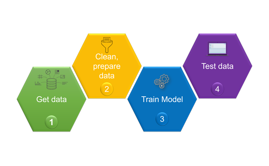
For building a powerful model, four steps were taken:
Overview of the machine learning pipeline and its workflow
The first step was the collection of data. For this, a training set consisting of 178 known individual substances was selected from various chemical classes, covering molecular weights (MW) ranging from 75.1 g/mol to 1131.3 g/mol, and computed octanol/water partition coefficients (SlogP) in the range of -7.53 to 13.98. Using the open source software KNIME and its extensions, molecular descriptors (e.g. MW, SlogP, topological polar surface area (TPSA)…) were computed for each substance. In addition, each substance was chromatographed with the CDS, generating 178 x 3 = 534 RF values. In the second step, the dataset was cleaned by filtering all descriptors for null variance. The third step included the training of the model. For this, the performance of three regressors was evaluated according to their capacity to predict the RF within the training set. The Random Forest, trained with 100 trees, yielded the best correlation coefficients R2 0.55, 0.72, and 0.64 for the LPDS, the MPDS, and the HPDS, respectively.
For testing of the model, a test set was created with 20 other substances. The suitability of the selected substances was verified by demonstrating that the chemical space of the test set was within the chemical space of the training set.
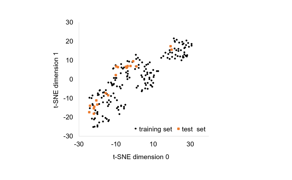
Chemical space (2D t-SNE projection) covered by the 178 chemicals belonging to the training set (black dots) and the 20 chemicals belonging to the test set (orange squares)
The model was used to predict the RF values of the compounds in the test set. Most predicted RF differ by less than 0.1 units from the measured values. RF in the MPDS and the HPDS are both predicted within the correct range and with very small errors, leading to R2 of 0.87, and 0.71, respectively. The variance for each individual prediction (LPDS, MPDS, and HPDS) remains smaller than 10%, except for a few compounds.
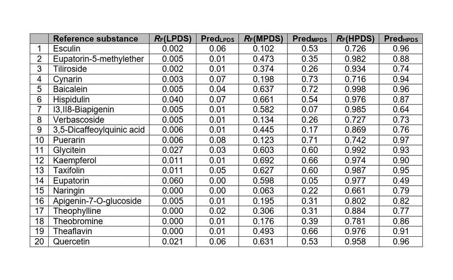
Measured and predicted RF values of the compounds in the test set
A reverse test was also performed. The query molecule defined by its RF values in LPDS, MPDS and HPDS was compared to the database for a number of rows (four each) matching the specified similarity. To calculate the similarity, the Euclidean distance was selected and the four nearer neighbors (most similar) were displayed in an additional column.
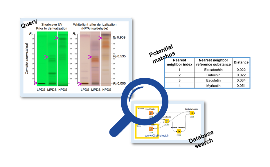
Use of the database for proposal of potential matches
Conclusion
The examples above illustrate the potential of the CDS and its combination with machine learning. In this study, RF values can be predicted, emphasizing that this feature is encoded within the chemical structure of the molecules. Moreover, the link between chemical structures and RF allows to generate a list of four molecules likely to correspond to an unknown zone in complex mixtures. This prediction would be even more useful, if additional data such as mass and UV-VIS spectra were added to the database.
[1] T.K.T. Do, M. Schmid, I. Trettin, M. Hänni, E. Reich, Complementary developing solvents for simpler and more powerful routine analysis by high-performance thin-layer chromatography, JPC – J. Planar Chromatogr. – Mod. TLC. (2022). https://doi.org/10.1007/s00764-022-00185-1.
[2] T.K.T. Do, I. Trettin, M. Hänni, E. Reich, Applying machine learning to the data obtained with the complementary developing solvents protocol, J. Liq. Chromatogr. Relat. Technol. (2023).
[3] T.K.T. Do, M. Schmid, M. Phanse, A. Charegaonkar, H. Sprecher, M. Obkircher, E. Reich, Development of the first universal mixture for use in system suitability tests for High-Performance Thin Layer Chromatography, J. Chromatogr. A. 1638 (2021) 461830. https://doi.org/10.1016/j.chroma.2020.461830.
Further information is available on request from the author(s).
Contact: Dr. Tiên Do, CAMAG, Sonnenmattstrasse 11, 4132 Muttenz, Switzerland, tien.do@camag.com